
In 1862, the Morrill Act allowed the federal government to expropriate over 10 million acres of tribal lands from Native communities, selling or developing them in order to fund public colleges. Over time, additional violence-backed treaties and land seizures ceded even more Indigenous lands to these “land-grant universities,” which continue to profit from these parcels.
But the Morrill Act is only one piece of legislation that connects land taken from Indigenous communities to land-grant universities. Over the past year, Grist looked at state trust lands, which are held and managed by state agencies for the schools’ continued benefit, and which total more than 500 million surface and subsurface acres across 21 states. We wanted to know how these acres, also stolen Indigenous land, are being used to fund higher education.
To do this, we needed to construct an original dataset.
- Grist located all state trust lands distributed through state enabling acts that currently send revenue to higher education institutions that also benefited from the Morrill Act.
- We identified their original Indigenous inhabitants and caretakers, and researched how much the United States would have paid for each parcel. The latter is based on an assessment of Indigenous territorial history, according to the U.S. Forest Service, associated with the land the parcels are on.
- We reconstructed more than 8.2 million acres of state trust parcels taken from 123 tribes, bands, and communities through 121 land cessions, a legal term for the surrendering of land. (It is important to note that land cession histories are incomplete and accurate only to the view of U.S. law and historical negotiations, not to Indigenous histories, epistemologies, or historic territories not captured by federal data.)
- The U.S. Forest Service dataset, which is based on the Schedule of Indian Land Cessions compiled by Charles Royce for the Eighteenth Annual Report of the Bureau of American Ethnology to the Secretary of the Smithsonian Institution (1896-1897), covers the period from 1787 to 1894.
This unique dataset was created through extensive spatial analysis that acquired, cleaned, and analyzed data from state repositories and departments across more than 14 states. We also reviewed historical financial records to supplement the dataset.
This information represents a snapshot of trust land parcels and activity present in November 2023. We encourage exploration of the database and caution that this snapshot is likely very different from state inventories 20, 50, or even 100 years ago. Since, to our knowledge, no other database of this kind exists — with this specific state trust land data benefitting land-grant universities — we are committed to making it publicly available and as robust as possible.
To identify what types of activities take place on state trust land parcels, we collected and compared state datasets on different kinds of land use. The activities in these data layers include, but are not limited to: active and inactive leases for coal, oil and gas, minerals, agriculture, grazing, commercial use, real estate, water, renewable energies, and easements. We then conducted spatial comparisons between these layers, explained further in Step 5 (see index below).
Users can also go to GitHub to view and download the code used to generate this dataset. The various functions used within the program can also be adapted and repurposed for analyzing other kinds of state trust lands — for example, those that send revenue to penitentiaries and detention centers, which a number of states do.
The database administrator can be contacted at [email protected].
If you republish this data or draw on it as a source for publication, cite as: Parazo Rose, Maria, et al. “Enabling Act Indigenous Land Parcels Database,” Grist.org, February 2024.
If you use this data for your own reporting, please be sure to credit Grist in the story and please send us a link.
Terminology
STL Parcel: State trust land parcels, or land granted to states through enabling acts. The word “parcel” refers to defined pieces of land that can range in size and are considered distinct units of property.
PLSS Number: The surveying method developed and used in the United States to plat, or divide, real property for sale and settling.
CRS System: A coordinate reference system that defines how a map projection in a GIS program relates to and represents real places on Earth. Deciding what CRS to use depends on the regional area of analysis.
Dataframe: A dataframe is a “two-dimensional” way of storing and manipulating tabular data, similar to a table with columns and rows.
REST API: An API, or application programming interface, is a type of software interface that allows users to communicate with a computer or system to retrieve information or perform a function. REST, also known as RESTful web services, stands for “representational state transfer” and has specific constraints. Systems with REST APIs optimize client-server interactions and can be scaled up efficiently.
Deduplication: Deduplication refers to a method of eliminating a dataset’s redundant data. In a secure data deduplication process, a deduplication assessment tool identifies extra copies of data and deletes them, so a single instance can then be stored. In our methodology, we deduplicated extra parcels, which we explain in further detail in Step 4.
Relevant Documents
Table 1: State Data Sources
Appendix A: Oklahoma and South Dakota processing
Steps
To reconstruct the redistribution of Indigenous lands and the comparative implications of their conversion to revenue for land-grant universities, we followed procedures that can be generally categorized in seven steps:
- Identify relevant university beneficiaries;
- Acquire data for STL parcels;
- Clean data for STL parcels;
- Merge data that came from various sources within a single state;
- Identify and join land use activity taking place on STL parcels;
- Join the parcel locations to Indigenous land cessions;
- Determine the price paid per acre; and
- Generate summary statistics
Identify university beneficiaries
We identified 14 universities in 14 states that initially benefited from the Morrill Act of 1862 and currently receive revenue benefits from state trust lands granted through enabling acts.
Initially, 30 states distributed funds to higher education institutions, including land-grant universities, according to their enabling acts. We contacted all 30 states via phone and email to confirm whether they had state trust lands that currently benefitted target institutions. Multiple states continue to distribute revenue generated from state trust lands to other higher education institutions, as well as K-12 schools. However, those states are not included in our dataset as the lands in question are outside the scope of this investigation.
In other words, multiple states have trust lands that produce revenue for institutions, but only 14 have trust lands that produce revenue for land-grant universities.
Data acquisition
Once we clarified which states had relevant STL parcels, the next step was to acquire the raw data of all state trust lands within that state so we could then filter for the parcels associated with land-grant institutions. We started by searching state databases, typically associated with their departments of natural resources, or the equivalent, to find data sources or maps. While most of the target states maintain online spatial data on land use and ownership, not all of that data is immediately available to download or access. For several states, we were able to scrape their online mapping platforms to access their REST servers and then query data through a REST API. For other states, we directly contacted their land management offices to get the most up-to-date information on STL parcels.
(Please see Table 1 for a list of the data sources referenced for each state, as well as all state-specific querying details.)
After acquiring the raw data, we researched which trust names were associated with the 14 identified universities. As mentioned above, each state maintains trust lands for multiple entities ranging from K-12 schools to penitentiaries, and each state has unique names for target beneficiaries in their mapping and financial data. We used these trust names to manually filter through the raw data and select only the parcels that currently send revenue to university beneficiaries and checked those names with state officials for accuracy.
Once identified and filtered, we reviewed that raw data to identify whether there were any additional fields that would be helpful to our schema (typically locational data of some kind, like PLSS, though this occasionally included activity or lease information) and included those fields as part of the data we extracted from state servers or the spatial files we were given, in addition to the geometric data that located and mapped the parcels themselves.
It’s important to note that we could not find information for 871 surface acres and 5,982 subsubsurface acres in Oklahoma, because they have yet to be digitally mapped or because of how they are sectioned on the land grid. We understand that this acreage does exist based on lists of activities kept by the state. However, those lists do not provide mappable data to fill these gaps. In order to complete reporting on Oklahoma, researchers will need to read and digitize physical maps and plats held by the state — labor this team was unable to provide during the project period.
Please also note that our dataset is partially incomplete due to the Montana Department of Natural Resources & Conservation’s delay in responding to a public records request by the time of publication. In the summer of 2023, we requested a complete dataset of state trust lands that send revenue to Montana State University. However, when we conducted a data review fact check with the Montana DNR this winter, they informed us that the data they supplied was incomplete and thus, inaccurate. We currently have a pending public records request that has yet to be returned.
(Please see Appendix A for specific notes on the data processing for OK.)
Data cleaning
When working with this data, one of the main considerations was that nearly all the data sources came in different and incompatible formats: The coordinate reference systems, or CRS, varied and had to be reprojected, the references to the trust names were inconsistent, and some files contained helpful fields, like location-specific identifiers or land use activity, while others were missing entire categories of information. Once we narrowed down the data we wanted, we cleaned and standardized the data, and sorted it into a common set of column names. This was particularly difficult for two states, Oklahoma and South Dakota, which required custom processing based on the format and quality of the initial data provided.
(Please see Appendix A for specific descriptions of the data processing for OK and SD.)
This process required a significant amount of state-specific formatting. This included processes such as:
- Querying certain fields in the source data to capture supplemental information, and then writing code to split or extract or take extra characters out of the values and assign the information to the appropriate columns.
- Processing files that, either because of the way we had to query servers or because of how state departments sent us data, were split up by activity type, in a way that allowed us to capture all of the information so it wouldn’t be lost in downstream processes.
- Creating functions that built off of information in the dataset to create new columns — like the net acres column, for example, for which we created an Idaho-specific function that calculated net acreage based on the percentage of state ownership, as indicated in the trust names.
Dataset merge
After all the data had been processed and cleaned, we needed to merge the various state files. The querying process ended up producing multiple files for each state, based on the number of trust names we were filtering for, as well as the rights type. Arizona, for example, had six trusts that sent revenue to the University of Arizona, each containing surface and subsurface acreage. Thus, we had 12 total AZ-specific files, since we generated six files, one for each trust, for surface acres, and another for subsurface acres.
These generated files are uniform to themselves, which means additional adjustments needed to be made for them to merge properly. So, before we merged all of a state’s files, we took each one — separated by rights type and trust name — and deleted the duplicate geometries that existed. We wanted to avoid repeating parcels that contained the same information because of the impact it would have on the acreage summaries, which is why we take a single file and delete information that contains the same rights type and trust name. In the process of geometric deduplication, we have taken particular care to aggregate any information that may be different — which, in our work, was mostly related to activity type. In these cases, if we deduplicated two parcels that were the same except for land use activity type that we noted in the raw data (not identified later in the activity match process), we combined both activities into a list in the activity field.
We can look at how the deduplication process plays out with an example in Montana and how it affects acreage. In our analysis, we report that Montana has 104,585.7 subsurface acres in its state trust land portfolio. However, that number refers to unique subsurface parcels in Montana. This is because we acquired the subsurface data as three separate files, identifying parcels affiliated with coal, oil and gas, or other minerals. Our process found parcels from different files that overlapped. So, we deleted the extra parcels and combined the activities. That way, we could use the main spreadsheet to determine that Montana’s subsurface acreage is broken down like this:
- Coal: 2,013.4 acres
- Oil and gas: 103,341.09 acres
- Other minerals: 1243.51 acres
- The sum of Montana’s subsurface acreage, by that analysis, is 106,598.
The difference in numbers is because some subsurface acres have multiple activities occurring on them. Our deduplication process identifies those acres with multiple activities and reduces that number to 104,585.7 acres.
As a note, we initially combined parcels that were geometric duplicates but had different rights types (for example, one had surface and the other had subsurface) to reflect that a parcel had both surface and subsurface rights. However, we found that this led to inaccuracies. In this final dataset, parcels have either surface or subsurface rights (or timber, in the case of Washington). Users should take care to note that instances of seemingly duplicated land parcels reflect this adjustment.
Prior to merging all state files into a single file, we calculated parcel acreage in the original source projection. Though most states record acreage of trust land parcels, several do not. So to assign acreage to parcels that had no area indicated and to create a consistent area measurement, we spatially calculated the acreage of all parcels through GIS to supplement the state-reported acres column. For accuracy, we calculated the acreage of the parcels in their initial source CRS and cross-referenced calculations with state agencies.
Mapping the land use activity
To identify what types of activity currently takes place on these parcels, we collected datasets on different kinds of land use from states, including, but not limited to, active and inactive leases for coal, oil and gas, minerals, agriculture, grazing, commercial use, real estate, water, renewable energies, and easements. We searched state databases or contacted land use offices to acquire spatial data, and we queried data through REST APIs. Initially, we called on state servers each time we ran our activity match operations, but the processing time was too inefficient, so we converted the majority of the datasets to shapefiles for faster processing.
It is important to note that states manage and track land use activity data in a variety of ways. Some states have different datasets for each type of activity, while some combine all land use activity into a single file. Some states indicate whether a certain lease or activity is presently active or not, some specify its precise status (prospecting, drilling, etc.), and some don’t include that information at all. Activities might be broadly classified as easement, agriculture, oil and gas, or coal — however, there might be a more specific description about its nature such as “Natural Gas Storage Operations,” “Access Road,” or “Offset Gas Well Pad.” Some states use numbers that require a key to interpret the activity. To accommodate these variations, we used the activity description that struck the best balance between being detailed and being clear, which either meant calling on the value of a specific column or titling the data layer as something general (“Oil and Gas”) and using that as the activity name. Users can look at the activity_match.py and state_data_sources.py files for further detail.
To identify how state trust land parcels are used, we gathered state datasets with spatial information on where land use activities take place. The data came as either points or polygons.
Users should note that, in the case of South Dakota, very few datasets on state land use activity were publicly accessible. Though we filed public records requests to obtain information, the state did not return our requests, leaving the activity fields for that state mostly empty of content apart from parcel locations.
Because there were so many data points in the information coming from states that were being matched against each row in the Grist dataset, we needed to find a way to expedite the process. Ultimately, we organized the activity datasets from each state into their own R-trees, tree data structures that are used to index multidimensional information, which allowed us to group together nearby parcels (which we will use from here on to mean polygons or points). For point data, we established bounding “envelopes” around each point to create the smallest appropriate polygon. In the diagram below, you can see an example of how nearby parcels are grouped together.
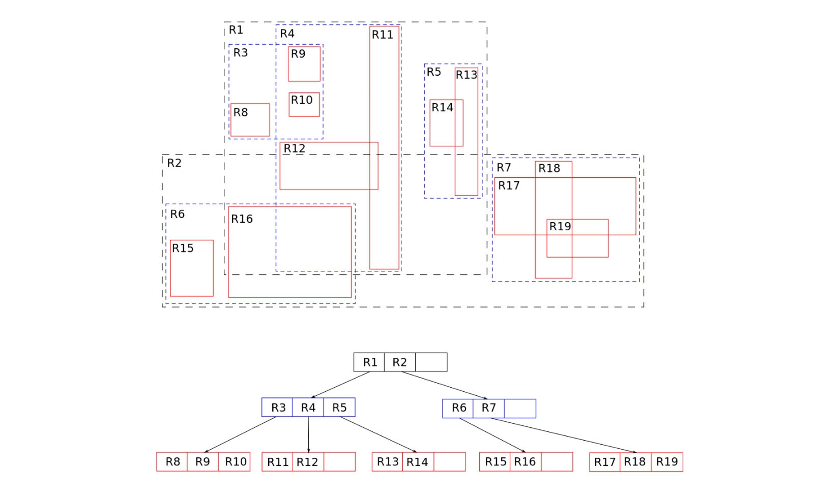
This data structure works by collecting nearby objects and organizing them with their minimum bounding rectangle. Then, one activity-set-turned-R-tree was compared to our trust land dataset at a time. In that process, a comparison looked at one Grist parcel through an activity’s R-tree, which is like a cascading way of identifying what parcels are close together. Whenever a query is conducted to compare another dataset against information in this R-tree, if a parcel does not intersect a given bounding rectangle, then it also cannot intersect any of the contained objects.
In other words, instead of comparing every parcel in our trust land dataset to every single other activity parcel in all of the state datasets, we are able to do much faster comparisons by looking at bigger areas and then narrowing down to more specific parcels when it’s relevant.
When the R-trees were established, we also had a process that looked at the distance from bounding rectangles in a state activity dataset’s tree structure and the closest points in the Grist state trust lands dataset. We only tracked that an activity was present on a trust land parcel if it overlapped and was the same geometric feature. That first method of geographic overlap test was called on Geopandas’ GeoSeries operations, seeing if a Grist-identified parcel contained, crossed, covered, intersected, touched, or was within an activity parcel. If any of the conditions were true, we “kept” that data, and marked that activity as present on the associated parcel.
We also had a second set of containment criteria that, if met, resulted in that activity being recorded as present. If we pulled in an activity parcel and, in comparing it to our trust land parcel dataset, found that it was the same geographic location, size (in acreage), and shape (via indices), we considered it to be a “duplicate parcel,” and recorded the presence of the relevant activity. We included all activities as a full list in the “activity” field associated with any given parcel.
Additionally, it is important to note that we made three kinds of modifications specific to the various land use activity layers, depending on the available data. First, there were some layers that had a field within the dataset indicating whether or not it was active. For those, we were able to assign an activity match only if that row was reported as active. Second, there were several layers that had relevant details we could use to supplement the activity description, which we included. Lastly, we only included activities relevant to the rights type associated with a parcel. If a parcel had subsurface rights, for example, then we did not indicate activities that may have happened on the surface — say, agriculture or road leases. Similarly, if a parcel had surface rights, we did not include subsurface activity, like minerals or oil and gas. We made additional adjustments to layers that contained “miscellaneous” data, containing activities that were surface or subsurface activities in the same layer. For those layers, we created a list of subsurface activity terms that would appear on surface-rights based parcels. This way, we ensured that the miscellaneous data layers could be read in their entirety, without misattributing activities.
Users can look at the activity_match.py and state_data_sources.py files for further detail.
Lastly, we generalized land use activities in order to create the data visualizations that accompany the story — specifically, the land use activity map. For user readability, we wanted to give an overarching perspective on how much land is used for some of the most prevalent activities. To do this, we manually reviewed all the values in the activity field and created lists that categorized specific activities into subsets of broader categories: fossil fuels, mining, timber, grazing, infrastructure, and renewable energy. With fossil fuels, for example, we included any activities that mentioned oil and gas wells or oil and gas fields, offset well pads, tank batteries, etc. Or, with infrastructure, we included activities that mentioned access roads or highways, pipelines, telecommunications systems, and power lines, among others. Some parcels are associated with multiple land uses, such as grazing cattle and oil production. In these cases, the acreage is counted for each practice. These lists then informed what parcels showed up in the six broad categories we featured in the land use map. (For further detail, users can explore the GitHub repo for our webpage interactives.)
Join to USFS Cession data
For a more comprehensive understanding of the dataset in its historical context, we joined the stl_dataset_extra_activities.geojson file to cession data from the U.S. Forest Service, or USFS. This enabled us to see the treaties or seizures that transferred “ownership” of land from tribal nations to the U.S. government. We have included steps here on how to conduct these processes in Excel and QGIS, which is a free and open access GIS software system. Similar operations exist in programs like ArcGIS. The steps to conduct the join can be found in our README file and in stl_dataset_extra_activities_plus_cessions.csv on GitHub.
Calculate financial information
Based on accounting of historical payments for treaties performed for legal proceedings undertaken by the Indian Claims Commission and the Court of Claims, we identified the price per acre for Royce cession areas underlying the parcels in the dataset. Using the average price per acre for cessions, we calculated the amount paid to Indigenous nations for each parcel.
Some parcels were overlapped by multiple cession areas. In those cases, to calculate the total paid to Indigenous nations for a parcel, we added the amount paid for each individual overlapping cession together.
To adjust for inflation we used CPI-based conversion factors for the U.S. dollars. For more on conversion factors, see here. We derived inflation adjustment factors from the tabular data available here.
For example, if Parcel A had 320 acres and overlaps Cession 1 where the U.S. bought the land for $0.05 per acre, part of Cession 2 that was seized and had no associated payment, and part of Cession 3 where the U.S. bought the land for $0.30 per acre, we calculated:
Price of parcel = (Total acreage x Price described in Cession 1) + (Total acreage x Price described in Cession 2 …) etc.
So:
Parcel A Price = (320*Cession1Price[$0.05]) + (320*Cession1Price[$0]) + (320*Cession1Price[$0.30])
Parcel A Price = $16 + $0 + 96
Price of parcel A = $112.00
A total of $112 is the price the federal government would have paid to tribal nations to acquire the land. In our dataset, the financial information on cessions has already been adjusted for inflation and can be considered as the amount paid in 2023 dollars.
Note that there are some Royce Cession ID numbers that we determined, after further research, were not actually land cessions. Rather, they described reservations created. We excluded these areas from our payment calculation.
We do not yet have financial information for cession ID 717 in Washington. The cession in question is 1,963.92 acres, and its absence means that the figures for price paid per acre or price paid per parcel are not complete for Washington.
It is also important to note that when documenting Indigenous land cessions in the continental United States, the Royce cession areas are extensive but incomplete. Although they are a standard source and are often treated as authoritative, they do not contain any cessions made after 1894 and likely miss or in other ways misrepresent included cessions prior to that time. We have made efforts to correct errors (primarily misdated cessions) when found, but have, in general, relied on the U.S. Forest Service’s digital files of the Royce dataset. A full review, revision, and expansion of the Royce land cession dataset is beyond the scope of this project.
Generate summary statistics
We wanted to aggregate this information so people could analyze the parcel data associated with a specific university or with a specific tribal nation. We generated two summary datasets: First, we combined all of the parcels by university to show their related tribes and cessions and how much the U.S. would have paid for these lands that they then gave to the universities. We created a second equivalent summary analysis that organizes information by present-day tribes and shows the associated universities, cessions, and payments. This step was accomplished after merging land cession and U.S. Forest Service data for better ease interacting with tribal leaders and impacted communities, as well as the removal of historic names, some of which are considered offensive today.
Please note that there were seven instances of tribes with similar names that we manually combined into a single row.
- Bridgeport Indian Colony, California, and Bridgeport Paiute Indian Colony of California
- Burns Paiute Tribe of the Burns Paiute Indian Colony of Oregon and Burns Paiute Tribe, Oregon
- Confederated Tribes and Bands of the Yakama Nation and Confederated Tribes and Bands of the Yakama Nation, Washington
- Nez Perce Tribe of Idaho and Nez Perce Tribe, Idaho
- Quinault Tribe of the Quinault Reservation, Washington, and Quinault Indian Nation, Washington
- Confederated Tribes of the Umatilla Reservation, Oregon, and Confederated Tribes of the Umatilla Indian Reservation, Oregon
- Shoshone-Bannock Tribes of the Fort Hall Reservation, Idaho, and Shoshone-Bannock Tribes of the Fort Hall Reservation of Idaho